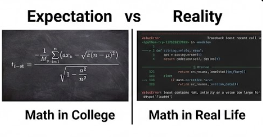
Hello World! The ML Script: Week 1
It was a long week full of maths, confusion, and a few “ohhh aisa bhi hota h !” moments. How so? Let me begin with the recap.
I began my ML journey by learning the prerequisite maths. I started following a dedicated maths curriculum specifically for ML algorithms, focusing on drawing conclusions by observing data rather than just memorizing formulas.
Fast forward to now, I have touched upon these topics:
Statistical Graphs / EDA Plots
Measures of Central Tendency (Mean, Median, Mode)
Measures of Spread (Dispersion)
Outlier Detection and Treatment
Probability Density Curves & Distribution Shapes
Hypothesis Testing (Z-test, T-test, Chi-Square, ANOVA)
I will be honest: learning this in a week != digesting it totally. I am a normal human, and I definitely have some "technical debt" in understanding all these concepts deeply. But I have a good grasp of the intuition now.
The list above is way too big to cover in a single blog. So, here are my Top 3 Learnings from this week.
1. Mean vs Median vs Mode (The Outlier War)
We all know what mean, median, and mode are. But the most important thing I learned is how Median is robust to outliers.
Outliers are data points that are abnormal with respect to the rest of the dataset. Usually, these are entries you want to clean up.
But there is a twist! Sometimes, outliers are valid. For example, imagine a dataset of college CGPAs vs. Salary Packages. There might be a student with a low CGPA who cracked a massive package because their interview was amazing. We can't drop this point—it's real data—even if it messes up the math, And this interview performance cannot really be converted into math. We simply can’t define how “good” an interview was in strict mathematical terms.
My takeaway:
Mean: Gets "dragged" by outliers. If one Student got a package 10x more than everyone else, the Mean shifts towards them, giving a false picture. (this also tells us that we should prioritize median package over mean package for college ranking )
Median: Is stubborn. It sits in the middle and ignores the noise at the edges.
Mode: Is also independent of outliers (unless your dataset is mostly outliers!). It’s the MVP for categorical data.
2. The "Z" vs "T" Confusion
This tripped me up the most. I learned two different tests that seem to do the exact same thing: The Z-Test and The T-Test.
I found out that the difference comes down to how much you know about the world (the Population):
Textbook Scenarios: If you know the Population Standard Deviation ($\sigma$) and have a huge sample size (n > 30), you use the Z-Test.
Real Life: In most ML projects, we don't know the population's true variance. We only have our small sample. In this case, the T-Test is the hero because it accounts for the uncertainty in our data.
I spent hours trying to understand why my z-score and p-value were coming out different when I calculated them manually using the z-score table, and in code using the ztest from the statsmodels library. In the end, I realized that to calculate a z-score, you need the standard deviation of the population, but I was not passing it to the ztest method from the statsmodels library.
Later, the documentation mentioned that it uses an estimation technique to calculate it using (ddof = 1), which was weird but understandable at the same time, as you never have information about the true population. So we use estimation techniques. But it is even more weird when someone doesn’t know the context.(Like I was Before Knowing the Truth)
3. Hypothesis Testing (Accept or Reject?)
I wouldn’t say this was "hard," but it was definitely confusing.
Hypothesis testing is how we mathematically decide if a pattern in our data is real or just luck.
Null Hypothesis ($H_0$): The boring option. "There is no difference" or "These two things are not related."
Alternate Hypothesis ($H_1$): The exciting option. "There is a significant difference" or "These things are related!"
The Confusing Part: When to reject $H_0$?
In math class, we use "Statistic Scores" and "Critical Regions" (confidence intervals).
- Example: If my T-score is 2.5 and my confidence interval is
[-1.96, 1.96], my score is outside the zone, so I reject the Null.
But in Python (using scipy.stats), we just use the P-Value, which is way easier:
The Golden Rule:
If P-value < Alpha (usually 0.05) → REJECT the Null (There is a relationship!)
Else → FAIL to Reject the Null (No relation found).
Think of the P-value as "The Probability that this happened by pure luck." If that probability is super low (less than 5%), we assume it wasn't luck—it’s real.
What's Next?
That was it for this week. There is obviously more depth to these topics (chi square , ANOVA), but I’m explaining what I actually understood.
For Week 2, I am moving from "Analyzing the Past" to "Predicting the Future." I will be focusing on Linear Regression. My goal is to understand the math behind the "Best Fit Line" before I just type model.fit().
See you in a week. If you don’t find a post, assume I’m slacking off (or stuck debugging).
Till then, let’s get scripting.